Fbprophet

Abstract

Forecasting is a common data science task that helps organizations with capacity planning, goal setting, and anomaly detection. Despite its importance, there are serious challenges associated with producing reliable and high quality forecasts – especially when there are a variety of time series and analysts with expertise in time series modeling are relatively rare. To address these challenges, we describe a practical approach to forecasting “at scale” that combines conﬁgurable models with analyst-in-the-loop performance analysis. We propose a modular regression model with interpretable parameters that can be intuitively adjusted by analysts with domain knowledge about the time series. We describe performance analyses to compare and evaluate forecasting procedures, and automatically ﬂag forecasts for manual review and adjustment. Tools that help analysts to use their expertise most eﬀectively enable reliable, practical forecasting of business time series.

摘要

预测是一项常见的数据科学任务，可帮助组织进行容量规划，目标设定和异常检测。尽管它具有重要性，但是在产生可靠和高质量的预测方面存在严重的挑战 - 特别是当存在各种时间序列时，具有时间序列建模专业知识的分析师相对较少。为了应对这些挑战，我们描述了一种实用的“大规模”预测方法，该方法将可配置模型与分析员在环性能分析相结合。我们提出了一个带有可解释参数的模块化回归模型，分析员可以通过对时间序列的领域知识直观地调整这些参数。我们描述了性能分析，以比较和评估预测程序，并自动进行人工审查和调整的预测。帮助分析师充分利用其专业知识的工具可以有效地实现对业务时间序列的可靠，实用的预测。

Keywords: Time Series, Statistical Practice, Nonlinear Regression

关键词：时间序列，统计实践，非线性回归

∗To whom correspondence should be addressed. †The authors contributed equally to this work.

*应该与谁通信。 †作者对这项工作的贡献相同。

1 Introduction

1简介

Forecasting is a data science task that is central to many activities within an organization. For instance, organizations across all sectors of industry must engage in capacity planning to eﬃciently allocate scarce resources and goal setting in order to measure performance relative to a baseline. Producing high quality forecasts is not an easy problem for either machines or for most analysts. We have observed two main themes in the practice of creating business forecasts. First, completely automatic forecasting techniques can be hard to tune and are often too inﬂexible to incorporate useful assumptions or heuristics. Second, the analysts responsible for data science tasks throughout an organization typically have deep domain expertise about the speciﬁc products or services that they support, but often do not have training in time series forecasting. Analysts who can produce high quality forecasts are thus quite rare because forecasting is a specialized skill requiring substantial experience.

预测是一项数据科学任务，对于组织内的许多活动至关重要。例如，所有行业部门的组织必须参与容量规划，以便有效地分配稀缺资源和目标设定，以便衡量相对于基线的绩效。对于任何一台机器或大多数分析师来说，生成高质量预测并不是一个容易的问题。我们在创建业务预测的实践中观察到两个主要主题。首先，完全自动的预测技术可能难以调整，并且通常太灵活，无法结合有用的假设或启发式。其次，负责整个组织的数据科学任务的分析师通常对他们支持的特定产品或服务拥有深厚的专业知识，但通常没有时间序列预测方面的培训。因此，能够产生高质量预测的分析师非常少见，因为预测是一项需要丰富经验的专业技能。

The result is that the demand for high quality forecasts often far outstrips the pace at which they can be produced. This observation is the motivation for the research we present here – we intend to provide some useful guidance for producing forecasts at scale, for several notions of scale.

结果是对高质量预测的需求往往远远超过它们的生产速度。这一观察结果是我们在此进行研究的动力 - 我们打算为几种规模概念提供一些有用的指导，以便大规模地进行预测。

The ﬁrst two types of scale we address are that business forecasting methods should be suitable for 1) a large number of people making forecasts, possibly without training in time series methods; and 2) a large variety of forecasting problems with potentially idiosyncratic features. In Section 3 we present a time series model which is ﬂexible enough for a wide range of business time series, yet conﬁgurable by non-experts who may have domain knowledge about the data generating process but little knowledge about time series models and methods.

我们解决的前两种规模是商业预测方法应该适合于1）大量人员进行预测，可能没有时间序列方法的培训; 2）各种具有潜在特殊功能的预测问题。在第3节中，我们提出了一个时间序列模型，该模型足够灵活，适用于广泛的业务时间序列，但可由非专家进行配置，这些非专家可能具有关于数据生成过程的领域知识，但对时间序列模型和方法知之甚少。

The third type of scale we address is that in most realistic settings, a large number of forecasts will be created, necessitating eﬃcient, automated means of evaluating and comparing them, as well as detecting when they are likely to be performing poorly. When hundreds or even thousands of forecasts are made, it becomes important to let machines do the hard work of model evaluation and comparison while eﬃciently using human feedback to ﬁx performance problems. In Section 4 we describe a forecast evaluation system that uses simulated historical forecasts to estimate out-of-sample performance and identify problematic forecasts for a human analyst to understand what went wrong and make necessary model adjustments.

我们要解决的第三种规模是，在大多数现实环境中，会产生大量的预测，需要有效的，自动化的方法来评估和比较它们，以及检测它们何时可能表现不佳。当进行数百甚至数千次预测时，让机器进行模型评估和比较的艰苦工作变得非常重要，同时有效地使用人工反馈来解决性能问题。在第4节中，我们描述了一个预测评估系统，该系统使用模拟的历史预测来估计样本外的性能，并为人类分析师确定有问题的预测，以了解出了什么问题并进行必要的模型调整。

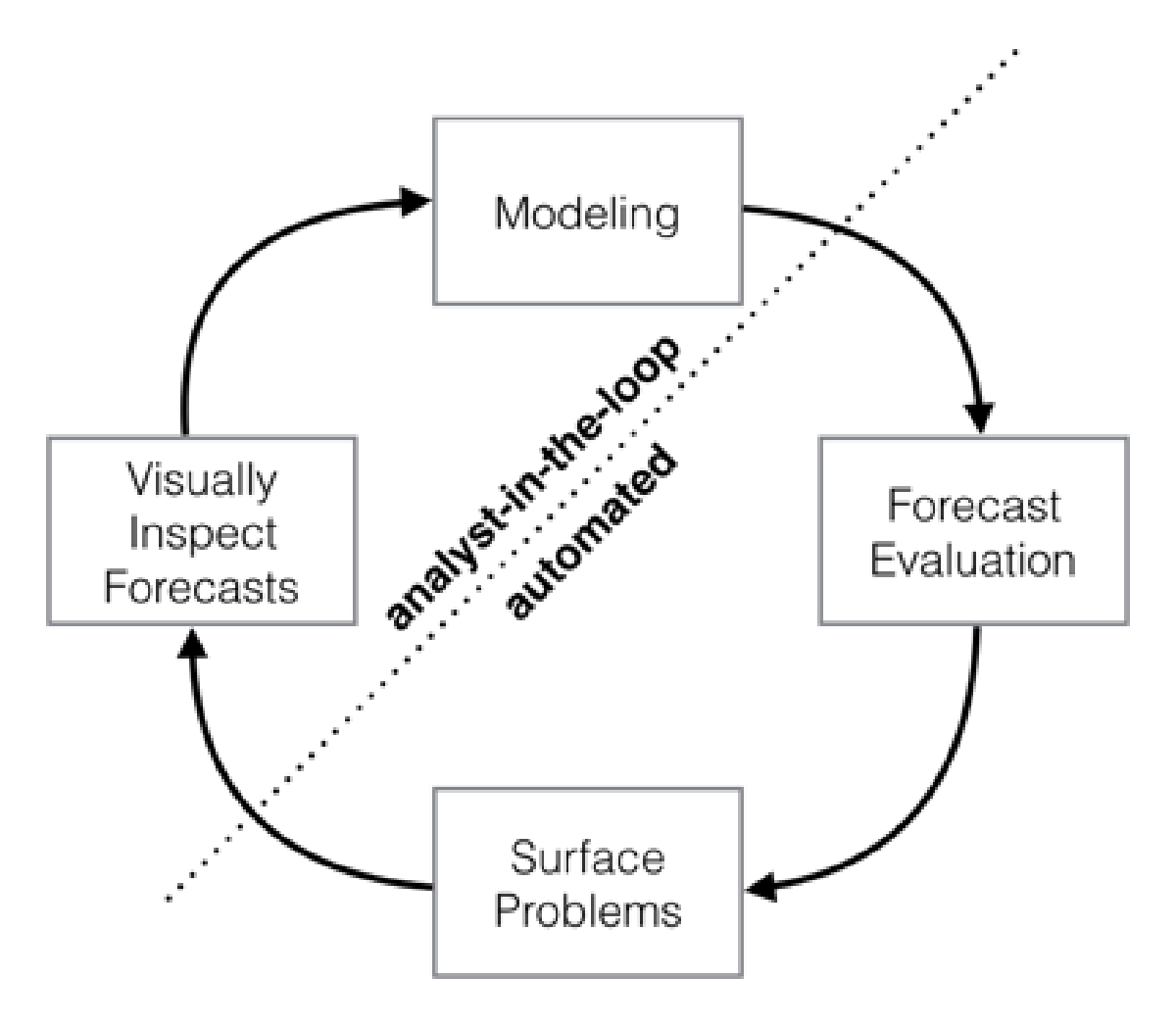
Figure 1: Schematic view of the analyst-in-the-loop approach to forecasting at scale, which best makes use of human and automated tasks.

图1：大规模预测的分析中在线方法的示意图，最好地利用人工和自动化任务。

It is worth noting that we are not focusing on the typical considerations of scale: computation and storage. We have found the computational and infrastructure problems of forecasting a large number of time series to be relatively straightforward – typically these ﬁtting procedures parallelize quite easily and forecasts are not diﬃcult to store in relational databases. The actual problems of scale we have observed in practice involve the complexity introduced by the variety of forecasting problems and building trust in a large number of forecasts once they have been produced.

值得注意的是，我们并没有关注规模的典型考虑因素：计算和存储。我们发现预测大量时间序列的计算和基础设施问题相对简单 - 通常这些设置过程非常容易并行化，并且预测不会存储在关系数据库中。我们在实践中观察到的实际规模问题涉及各种预测问题引入的复杂性，并且一旦产生预测就会在大量预测中建立信任。

We summarize our analyst-in-the-loop approach to business forecasting at scale in Fig. 1. We start by modeling the time series using a ﬂexible speciﬁcation that has a straightforward human interpretation for each of the parameters. We then produce forecasts for this model and a set of reasonable baselines across a variety of historical simulated forecast dates, and evaluate forecast performance. When there is poor performance or other aspects of the forecasts warrant human intervention, we ﬂag these potential problems to a human analyst in a prioritized order. The analyst can then inspect the forecast and potentially adjust the model based on this feedback.

我们在图1中概括了大规模业务预测的分析员在循环方法。我们首先使用灵活的规范对时间序列进行建模，该规范对每个参数都有直接的人工解释。然后，我们针对此模型生成预测，并在各种历史模拟预测日期生成一组合理的基线，并评估预测性能。当表现不佳或预测的其他方面需要人为干预时，我们会按照优先顺序将这些潜在问题提交给人类分析师。然后，分析师可以检查预测，并可能根据此反馈调整模型。

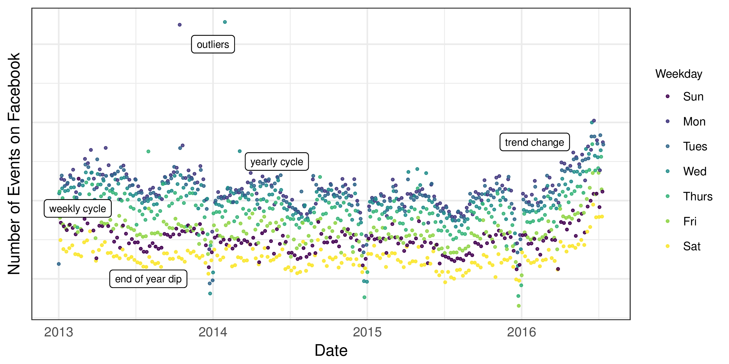
Figure 2: The number of events created on Facebook. There is a point for each day, and points are color-coded by day-of-week to show the weekly cycle. The features of this time series are representative of many business time series: multiple strong seasonalities, trend changes, outliers, and holiday eﬀects.

图2：在Facebook上创建的事件数。每天都有一个点，点数按星期显示颜色，以显示每周周期。这个时间序列的特征代表了许多商业时间序列：多个强烈的季节性，趋势变化，异常值和假期效应。

2 Features of Business Time Series

2营业时间序列的特点

There is a wide diversity of business forecasting problems, however there are some features common to many of them. Fig. 2 shows a representative Facebook time series for Facebook Events. Facebook users are able to use the Events platform to create pages for events, invite others, and interact with events in a variety of ways. Fig. 2 shows daily data for the number of events created on Facebook. There are several seasonal eﬀects clearly visible in this time series: weekly and yearly cycles, and a pronounced dip around Christmas and New Year. These types of seasonal eﬀects naturally arise and can be expected in time series generated by human actions. The time series also shows a clear change in trend in the last six months, which can arise in time series impacted by new products or market changes. Finally, real datasets often have outliers and this time series is no exception.

存在各种各样的业务预测问题，但是它们中的许多都有一些共同的特征。图2显示了Facebook Events的代表性Facebook时间序列。Facebook用户可以使用Events平台为事件创建页面，邀请其他人以及以各种方式与事件交互。图2显示了在Facebook上创建的事件数量的每日数据。在这个时间序列中可以清楚地看到几种季节性影响：每周和每年周期，以及圣诞节和新年期间的明显下降。这些类型的季节性影响自然会产生，并且可以在人类行为产生的时间序列中预期。时间序列也显示了过去六个月的趋势明显变化，这可能会受到新产品或市场变化影响的时间序列的影响。最后，真实的数据集通常有异常值，这个时间序列也不例外。

This time series provides a useful illustration of the diﬃculties in producing reasonable forecasts with fully automated methods. Fig. 3 shows forecasts using several automated procedures from the forecast package in R, described in Hyndman et al. (2007). Forecasts were made at three points in the history, each using only the portion of the time series up to that point to simulate making a forecast on that date. The methods in the ﬁgure are: auto.arima, which ﬁts a range of ARIMA models and automatically selects the best one; ets, which ﬁts a collection of exponential smoothing models and selects the best (Hyndman et al. 2002); snaive, a random walk model that makes constant predictions with weekly seasonality (seasonal naive); and tbats, a TBATS model with both weekly and yearly seasonalities (De Livera et al. 2011).

这个时间序列提供了一个有用的例子，说明了用全自动方法产生合理预测的困难。图3显示了使用来自R中的预测包的若干自动程序的预测，如Hyndman等人所述。（2007年）。在历史记录中的三个点进行了预测，每个点仅使用截至该点的时间序列部分来模拟在该日期进行预测。图中的方法是：auto.arima，它包含一系列ARIMA模型并自动选择最佳模型; ets，它是指数平滑模型的集合并选择最好的（Hyndman et al.2002）; snaive，随机游走模型，每周季节性（季节性幼稚）进行持续预测;和tbats，TBATS模型，每周和每年的季节性（De Livera et al.2011）。

The methods in Fig. 3 generally struggle to produce forecasts that match the characteristics of these time series. The automatic ARIMA forecasts are prone to large trend errors when there is a change in trend near the cutoﬀ period and they fail to capture any seasonality.1 The exponential smoothing and seasonal naive forecasts capture weekly seasonality but miss longer-term seasonality. All of the methods overreact to the end-of-year dip because they do not adequately model yearly seasonality.

图3中的方法通常很难产生与这些时间序列的特征相匹配的预测。当cuto ff时期附近的趋势发生变化并且未能捕捉任何季节性时，自动ARIMA预测容易出现大的趋势误差.1指数平滑和季节性天真预测捕获每周季节性但错过长期季节性。所有这些方法都对年末下降反应过度，因为它们没有充分模拟年度季节性。

When a forecast is poor, we wish to be able to tune the parameters of the method to the problem at hand. Tuning these methods requires a thorough understanding of how the underlying time series models work. The ﬁrst input parameters to automated ARIMA, for instance, are the maximum orders of the diﬀerencing, the auto-regressive components, and the moving average components. A typical analyst will not know how to adjust these orders to avoid the behavior in Fig. 3 – this is the type of expertise that is hard to scale.

当预测很差时，我们希望能够将方法的参数调整到手头的问题。调整这些方法需要彻底了解基础时间序列模型的工作原理。例如，自动ARIMA的第一个输入参数是差异的最大阶数，自动回归分量和移动平均分量。典型的分析师不知道如何调整这些订单以避免图3中的行为 - 这是难以扩展的专业类型。

3 The Prophet Forecasting Model

3先知预测模型

We now describe a time series forecasting model designed to handle the common features of business time series seen in Fig. 2. Importantly, it is also designed to have intuitive parameters that can be adjusted without knowing the details of the underlying model. This is necessary for the analyst to eﬀectively tune the model as described in Fig. 1. Our implementation is available as open source software in Python and R, called Prophet 1ARIMA models are capable of including seasonal covariates, but adding these covariates leads to extremely long ﬁtting times and requires modeling expertise that many forecasting novices would not have.

我们现在描述一个时间序列预测模型，旨在处理图2中所见的业务时间序列的共同特征。重要的是，它还具有直观的参数，可以在不知道底层模型细节的情况下进行调整。这对于分析师来说是必要的，如图1所示，有效地调整模型。我们的实现可以作为Python和R中的开源软件使用，称为Prophet 1ARIMA模型能够包含季节性协变量，但添加这些协变量会导致极长的安装时间，并且需要许多预测新手不具备的建模专业知识。

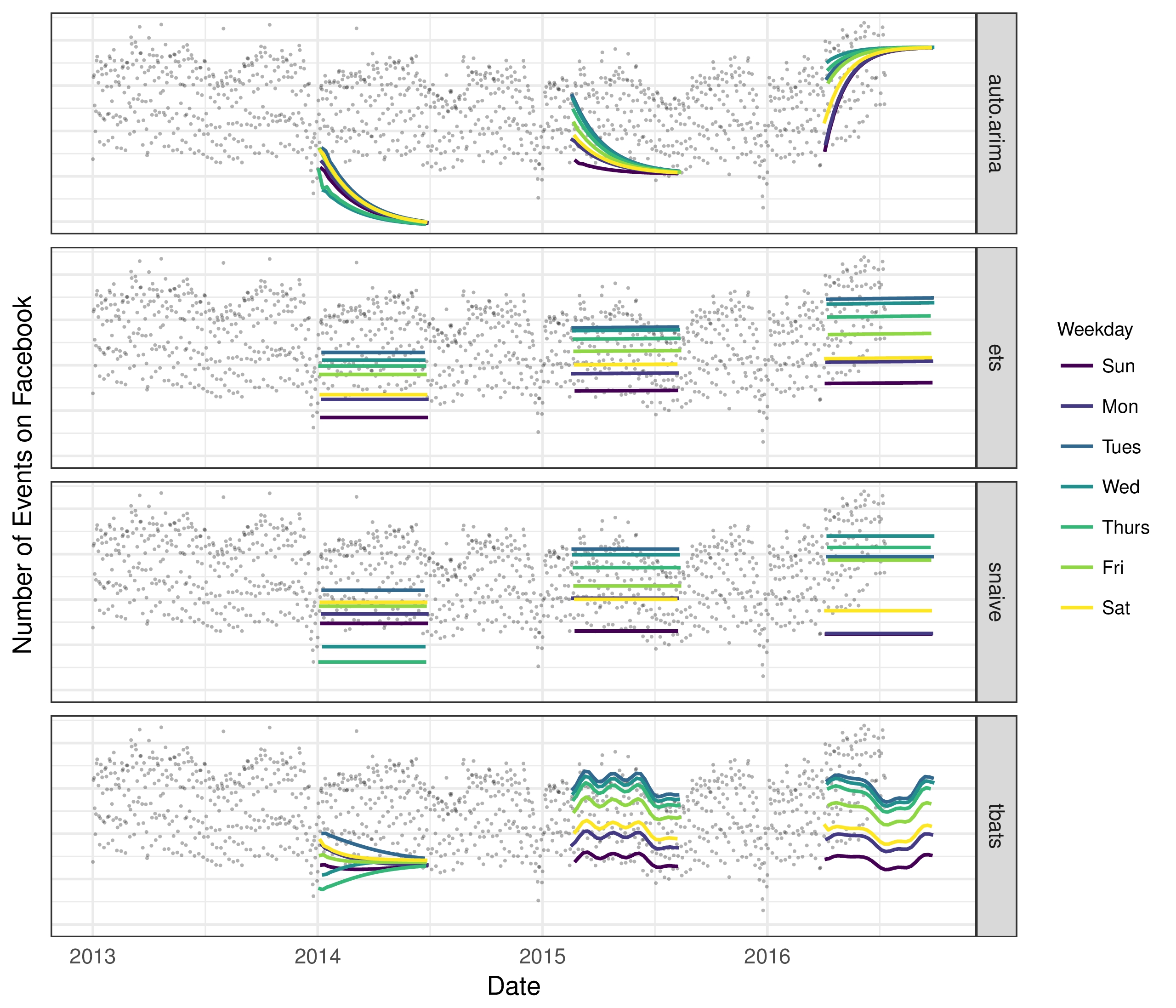
Figure 3: Forecasts on the time series from Fig. 2 using a collection of automated forecasting procedures. Forecasts were made at three illustrative points in the history, each using only the portion of the time series up to that point. Forecasts for each day are grouped and colored by day-of-week to visualize weekly seasonality. We removed the outliers during plotting to allow for more vertical space in the ﬁgure.

图3：使用一系列自动预测程序对图2中的时间序列进行预测。预测是在历史中的三个说明点进行的，每个点仅使用到该点的时间序列的部分。每天的预测按星期分组并着色，以显示每周季节性。我们在绘图过程中删除了异常值，以便在图中留出更多的垂直空间。

(https://facebook.github.io/prophet/).

（https://facebook.github.io/prophet/）。

We use a decomposable time series model (Harvey & Peters 1990) with three main model components: trend, seasonality, and holidays. They are combined in the following equation:

我们使用可分解的时间序列模型（Harvey＆Peters 1990），其中包含三个主要模型组件：趋势，季节性和假期。它们按以下等式组合： \(y(t)=g(t)+s(t)+h(t)+\epsilon_t.\)

Here g(t) is the trend function which models non-periodic changes in the value of the time series, s(t) represents periodic changes (e.g., weekly and yearly seasonality), and h(t) represents the eﬀects of holidays which occur on potentially irregular schedules over one or more days. The error term \(\epsilon_t\) represents any idiosyncratic changes which are not accommodated by the model; later we will make the parametric assumption that \(\epsilon_t\) is normally distributed.

这里g（t）是趋势函数，它模拟时间序列值的非周期性变化，s（t）代表周期性变化（例如，每周和每年季节性），h（t）代表假期的影响。在一天或多天内发生在可能不正常的时间表上。错误术语 \(\epsilon_t\)表示模型不能满足的任何特殊变化;稍后我们将做出 \(\epsilon_t\)正态分布的参数假设。

This speciﬁcation is similar to a generalized additive model (GAM) (Hastie & Tibshirani 1987), a class of regression models with potentially non-linear smoothers applied to the regressors. Here we use only time as a regressor but possibly several linear and non-linear functions of time as components. Modeling seasonality as an additive component is the same approach taken by exponential smoothing (Gardner 1985). Multiplicative seasonality, where the seasonal eﬀect is a factor that multiplies g(t), can be accomplished through a log transform.

该规范类似于广义加性模型（GAM）（Hastie＆Tibshirani 1987），这是一类回归模型，具有应用于回归量的潜在非线性平滑器。这里我们只使用时间作为回归量，但可能使用时间的几个线性和非线性函数作为分量。将季节性建模作为附加成分与指数平滑相同（Gardner 1985）。季节性效应是乘以g（t）的因子的乘法季节性可以通过对数变换来实现。

The GAM formulation has the advantage that it decomposes easily and accommodates new components as necessary, for instance when a new source of seasonality is identiﬁed. GAMs also ﬁt very quickly, either using backﬁtting or L-BFGS (Byrd et al. 1995) (we prefer the latter) so that the user can interactively change the model parameters.

GAM配方的优点在于它可以轻松分解并根据需要容纳新组分，例如在确定新的季节性来源时。GAM也很快，无论是使用反向装配还是L-BFGS（Byrd等人1995）（我们更喜欢后者），以便用户可以交互式地改变模型参数。

We are, in eﬀect, framing the forecasting problem as a curve-ﬁtting exercise, which is inherently diﬀerent from time series models that explicitly account for the temporal dependence structure in the data. While we give up some important inferential advantages of using a generative model such as an ARIMA, this formulation provides a number of practical advantages:

实际上，我们将预测问题定义为曲线拟合练习，这与时间序列模型本质上不同，时间序列模型明确地说明了数据中的时间依赖结构。虽然我们放弃了使用ARIMA等生成模型的一些重要的推理优势，但这种配方提供了许多实际优势：

– Flexibility: We can easily accommodate seasonality with multiple periods and let the analyst make diﬀerent assumptions about trends.

- 灵活性：我们可以轻松地适应多个时期的季节性，让分析师对趋势做出不同的假设。

– Unlike with ARIMA models, the measurements do not need to be regularly spaced, and we do not need to interpolate missing values e.g. from removing outliers.

- 与ARIMA模型不同，测量不需要定期间隔，我们不需要插入缺失值，例如：从删除异常值。

– Fitting is very fast, allowing the analyst to interactively explore many model speciﬁcations, for example in a Shiny application (Chang et al. 2015).

- 拟合非常快，允许分析人员以交互方式探索许多模型规范，例如在Shiny应用程序中（Chang et al.2015）。

– The forecasting model has easily interpretable parameters that can be changed by the analyst to impose assumptions on the forecast. Moreover, analysts typically do have experience with regression and are easily able to extend the model to include new components.

- 预测模型具有易于解释的参数，分析师可以更改这些参数以对预测进行假设。此外，分析师通常具有回归经验，并且能够轻松扩展模型以包含新组件。

Automatic forecasting has a long history, with many methods tailored to speciﬁc types of time series (Tashman & Leach 1991, De Gooijer & Hyndman 2006). Our approach is driven by both the nature of the time series we forecast at Facebook (piecewise trends, multiple seasonality, ﬂoating holidays) as well as the challenges involved in forecasting at scale.

自动预测历史悠久，有许多方法适合特定类型的时间序列（Tashman＆Leach 1991，De Gooijer＆Hyndman 2006）。我们的方法是由我们在Facebook预测的时间序列的性质（分段趋势，多重季节性，假期）以及大规模预测所涉及的挑战所驱动的。

3.1 The Trend Model

3.1趋势模型

We have implemented two trend models that cover many Facebook applications: a saturating growth model, and a piecewise linear model.

我们已经实现了两个涵盖许多Facebook应用程序的趋势模型：饱和增长模型和分段线性模型。

3.1.1 Nonlinear, Saturating Growth

3.1.1非线性，饱和增长

For growth forecasting, the core component of the data generating process is a model for how the population has grown and how it is expected to continue growing. Modeling growth at Facebook is often similar to population growth in natural ecosystems (e.g., Hutchinson 1978), where there is nonlinear growth that saturates at a carrying capacity. For example, the carrying capacity for the number of Facebook users in a particular area might be the number of people that have access to the Internet. This sort of growth is typically modeled using the logistic growth model, which in its most basic form is

对于增长预测，数据生成过程的核心组成部分是人口增长方式以及预期如何继续增长的模型。Facebook的模型增长通常类似于自然生态系统中的人口增长（例如，Hutchinson 1978），其中非线性增长在承载能力下饱和。例如，特定区域中Facebook用户数量的承载能力可能是可以访问互联网的人数。这种增长通常使用逻辑增长模型建模，其最基本的形式是 \(g(t)=\frac{C}{1+ exp(-k(t-m))}\)

with C the carrying capacity, k the growth rate, and m an oﬀset parameter.

C为承载能力，k为增长率，m为设定参数。

There are two important aspects of growth at Facebook that are not captured in (2). First, the carrying capacity is not constant – as the number of people in the world who have access to the Internet increases, so does the growth ceiling. We thus replace the ﬁxed capacity C with a time-varying capacity C(t). Second, the growth rate is not constant. New products can profoundly alter the rate of growth in a region, so the model must be able to incorporate a varying rate in order to ﬁt historical data.

Facebook增长有两个重要方面，未在（2）中捕获。首先，承载能力不是恒定的 - 随着世界上可以访问互联网的人数增加，增长上限也增加。因此，我们用随时间变化的容量C（t）代替固定容量C.其次，增长率不是恒定的。新产品可以深刻地改变一个地区的增长率，因此该模型必须能够包含不同的速率以便提供历史数据。

We incorporate trend changes in the growth model by explicitly deﬁning changepoints where the growth rate is allowed to change. Suppose there are S changepoints at times\(S_j\) , j = 1,. , S. We deﬁne a vector of rate adjustments\(\delta \in \mathbb{R}^{S}\) , where\(\delta_j\) is the change in rate that occurs at time \(S_j\) The rate at any time t is then the base rate k, plus all of the adjustments up to that point: k + : This is represented more cleanly by deﬁning a vector a(t) 0, 1 such that

我们通过明确定义允许增长率变化的变化点，将增长模型中的趋势变化纳入其中。假设，j = 1，有时有S个变化点。，S。我们定义了一个速率调整的向量，其中是在时发生的速率变化。任何时间t的速率都是基本速率k加上到那一点的所有调整：k + ：通过定义向量a（t） 0,1 这样表示得更干净

The rate at time t is then k + a(t) . When the rate k is adjusted, the oﬀset parameter m must also be adjusted to connect the endpoints of the segments. The correct adjustment at changepoint j is easily computed as

在时间t的速率则是k + a（t）。当调整速率k时，还必须调整o ff设置参数m以连接段的端点。变换点j处的正确调整很容易计算为

The piecewise logistic growth model is then

然后是分段后勤增长模型

An important set of parameters in our model is C(t), or the expected capacities of the system at any point in time. Analysts often have insight into market sizes and can set these accordingly. There may also be external data sources that can provide carrying capacities, such as population forecasts from the World Bank.

我们模型中的一组重要参数是C（t），或系统在任何时间点的预期容量。分析师通常可以深入了解市场规模，并可以相应地设置这些。可能还有外部数据源可以提供承载能力，例如世界银行的人口预测。

The logistic growth model presented here is a special case of generalized logistic growth curves, which is only a single type of sigmoid curve. Extensions of this trend model to other families of curves is straightforward.

这里给出的逻辑增长模型是广义逻辑增长曲线的一个特例，它只是一种类型的S形曲线。将此趋势模型扩展到其他曲线族是很简单的。

3.1.2 Linear Trend with Changepoints

3.1.2带变化点的线性趋势

For forecasting problems that do not exhibit saturating growth, a piece-wise constant rate of growth provides a parsimonious and often useful model. Here the trend model is

对于没有表现出饱和增长的预测问题，分段的恒定增长率提供了一种简约且通常有用的模型。这里的趋势模型是

where as before k is the growth rate, δ has the rate adjustments, m is the oﬀset parameter, and is set to to make the function continuous.

其中k是生长速率，δ是速率调整，m是o ff设置参数，设置为以使函数连续。

3.1.3 Automatic Changepoint Selection

3.1.3自动变更点选择

The changepoints could be speciﬁed by the analyst using known dates of product launches and other growth-altering events, or may be automatically selected given a set of candidates. Automatic selection can be done quite naturally with the formulation in (3) and (4) by putting a sparse prior on δ.

的变更点可以由分析师使用已知的产品发布日期和其他增长改变事件来指定，也可以在给定一组候选人的情况下自动选择。通过在δ上放置稀疏先验，可以使用（3）和（4）中的公式非常自然地进行自动选择。

We often specify a large number of changepoints (e.g., one per month for a several year history) and use the prior Laplace(0 ). The parameter τ directly controls the ﬂexibility of the model in altering its rate. Importantly, a sparse prior on the adjustments δ has no impact on the primary growth rate k, so as τ goes to 0 the ﬁt reduces to standard (not-piecewise) logistic or linear growth.

我们经常指定大量的变更点（例如，几年历史中每月一个）并使用先前的拉普拉斯（0 ）。参数τ直接控制模型在改变其速率方面的灵活性。重要的是，在调整δ之前的稀疏先验对初级生长速率k没有影响，因此当τ变为0时，该结果减少到标准（非分段）逻辑或线性增长。

3.1.4 Trend Forecast Uncertainty

3.1.4趋势预测不确定性

When the model is extrapolated past the history to make a forecast, the trend will have a constant rate. We estimate the uncertainty in the forecast trend by extending the generative model forward. The generative model for the trend is that there are S changepoints over a history of T points, each of which has a rate change Laplace(0 ). We simulate future rate changes that emulate those of the past by replacing τ with a variance inferred from data. In a fully Bayesian framework this could be done with a hierarchical prior on τ to obtain its posterior, otherwise we can use the maximum likelihood estimate of the rate scale parameter: λ = 1 =1 . Future changepoints are randomly sampled in such a way that the average frequency of changepoints matches that in the history: = 0 w.p. Laplace(0 ) w.p. ST .

当模型推断出历史记录以进行预测时，趋势将具有恒定的速率。我们通过扩展生成模型来估计预测趋势的不确定性。该趋势的生成模型是在T点历史上存在S个变化点，每个T点具有速率变化 Laplace（0 ）。我们通过用从数据推断的方差替换τ来模拟模拟过去的未来速率变化。在完全贝叶斯框架中，这可以通过τ上的分层先验来完成以获得其后验，否则我们可以使用速率尺度参数的最大似然估计：λ= 1 = 1 。对未来的变化点进行随机抽样，使得变化点的平均频率与历史中的变化点匹配：= 0 w.p. 拉普拉斯（0 ）w.p。 ST。

We thus measure uncertainty in the forecast trend by assuming that the future will see the same average frequency and magnitude of rate changes that were seen in the history. Once λ has been inferred from the data, we use this generative model to simulate possible future trends and use the simulated trends to compute uncertainty intervals.

因此，我们假设未来将看到历史中看到的相同的平均频率和速率变化幅度，从而衡量预测趋势的不确定性。一旦从数据中推断出λ，我们使用该生成模型来模拟可能的未来趋势，并使用模拟趋势来计算不确定性区间。

The assumption that the trend will continue to change with the same frequency and magnitude as it has in the history is fairly strong, so we do not expect the uncertainty intervals to have exact coverage. They are, however, a useful indication of the level of uncertainty, and especially an indicator of overﬁtting. As τ is increased the model has more ﬂexibility in ﬁtting the history and so training error will drop. However, when projected forward this ﬂexibility will produce wide uncertainty intervals.

假设趋势将继续以与历史相同的频率和幅度发生变化，这种假设相当强烈，因此我们不希望不确定性区间具有精确的覆盖范围。然而，它们是不确定性水平的有用指示，尤其是过度配置的指标。随着τ的增加，模型在拟合历史时具有更大的灵活性，因此训练误差将会下降。然而，当向前推进时，这种灵活性将产生广泛的不确定性区间。

3.2 Seasonality

3.2季节性

Business time series often have multi-period seasonality as a result of the human behaviors they represent. For instance, a 5-day work week can produce eﬀects on a time series that repeat each week, while vacation schedules and school breaks can produce eﬀects that repeat each year. To ﬁt and forecast these eﬀects we must specify seasonality models that are periodic functions of t.

由于他们所代表的人类行为，商业时间系列通常具有多周期季节性。例如，一个为期5天的工作周可以产生每周重复的时间序列的效果，而假期安排和学校休息可以产生每年重复的效果。为了确定和预测这些影响，我们必须指定作为t的周期函数的季节性模型。

We rely on Fourier series to provide a ﬂexible model of periodic eﬀects (Harvey & Shephard 1993). Let P be the regular period we expect the time series to have (e.g. P = 365.25 for yearly data or P = 7 for weekly data, when we scale our time variable in days). We can approximate arbitrary smooth seasonal eﬀects with

我们依靠傅立叶级数来提供周期性效应的灵活模型（Harvey＆Shephard 1993）。设P是我们期望时间序列的常规周期（例如，对于每年数据P = 365.25或每周数据P = 7，当我们以天为单位缩放时间变量时）。我们可以近似任意平滑的季节性效果

a standard Fourier series2. Fitting seasonality requires estimating the 2N parameters β = [a1 1,. , aN , bN ]ᵀ. This is done by constructing a matrix of seasonality vectors for each 2The intercept term can be left out because we are simultaneously ﬁtting a trend component.

标准的傅里叶级数2。拟合季节性需要估计2N参数β= [a1 1，。，aN，bN]ᵀ。这是通过为每个2构建季节性向量矩阵来完成的。拦截项可以省略，因为我们同时处理趋势分量。

value of t in our historical and future data, for example with yearly seasonality and N = 10,

我们的历史和未来数据中的t值，例如年度季节性和N = 10，

The seasonal component is then

然后是季节性成分

In our generative model we take Normal(0 2) to impose a smoothing prior on the seasonality.

在我们的生成模型中，我们采用 Normal（0 2）对季节性进行平滑处理。

Truncating the series at N applies a low-pass ﬁlter to the seasonality, so increasing N allows for ﬁtting seasonal patterns that change more quickly, albeit with increased risk of overﬁtting. For yearly and weekly seasonality we have found N = 10 and N = 3 respectively to work well for most problems. The choice of these parameters could be automated using a model selection procedure such as AIC.

在N处截断该系列会对季节性应用低通滤波器，因此增加N允许配置变化更快的季节性模式，尽管过度安装的风险增加。对于每年和每周的季节性，我们发现N = 10和N = 3分别对大多数问题都有效。可以使用诸如AIC的模型选择程序来自动选择这些参数。

3.3 Holidays and Events

3.3假期和活动

Holidays and events provide large, somewhat predictable shocks to many business time series and often do not follow a periodic pattern, so their eﬀects are not well modeled by a smooth cycle. For instance, Thanksgiving in the United States occurs on the fourth Thursday in November. The Super Bowl, one of the largest televised events in the US, occurs on a Sunday in January or February that is diﬃcult to declare programmatically. Many countries around the world have major holidays that follow the lunar calendar. The impact of a particular holiday on the time series is often similar year after year, so it is important to incorporate it into the forecast.

假期和事件对许多业务时间序列提供了大的，有些可预测的冲击，并且通常不遵循周期性模式，因此它们的影响不能通过平稳循环很好地建模。例如，美国的感恩节发生在11月的第四个星期四。超级碗是美国最大的电视转播事件之一，发生在1月或2月的一个星期天，很难以编程方式宣布。世界上许多国家都有农历节日。特定假期对时间序列的影响通常年复一年，因此将其纳入预测非常重要。

We allow the analyst to provide a custom list of past and future events, identiﬁed by the event or holiday’s unique name, as shown in Table 1. We include a column for country in order to keep a country-speciﬁc list of holidays in addition to global holidays. For a given forecasting problem we use the union of the global set of holidays and the country-speciﬁc ones.

我们允许分析师提供过去和未来事件的自定义列表，由事件或假日的唯一名称标识，如表1所示。我们为国家/地区添加了一个列，以便在全球假期之外保留国家/地区特定的假期列表。对于给定的预测问题，我们使用全球假日集和国家特定假期的联合。

Incorporating this list of holidays into the model is made straightforward by assuming that the eﬀects of holidays are independent. For each holiday i, let be the set of past and future dates for that holiday. We add an indicator function representing whether time t is during holiday i, and assign each holiday a parameter which is the corresponding change in the forecast. This is done in a similar way as seasonality by generating a matrix of regressors

通过假设假期的影响是独立的，将这个假期列表纳入模型是直截了当的。对于每个假期我，让成为该假期的过去和未来日期的集合。我们添加一个指示函数，表示时间t是否在假期i期间，并为每个假期分配一个参数，这是预测中的相应变化。这通过生成回归量矩阵以与季节性类似的方式完成

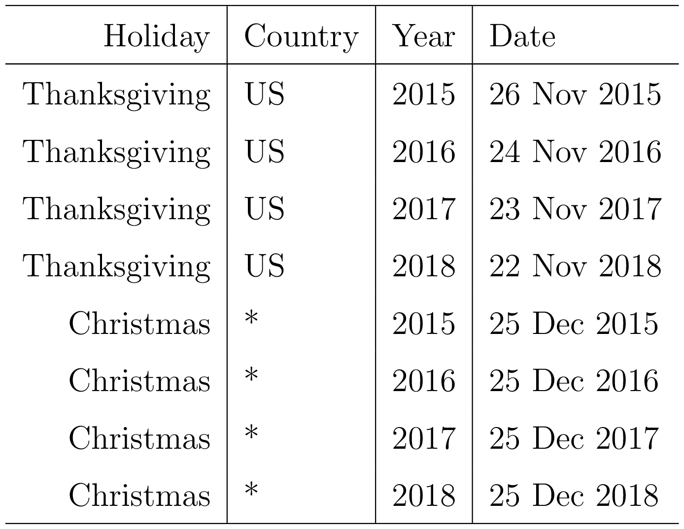
Table 1: An example list of holidays. Country is speciﬁed because holidays may occur on diﬀerent days in diﬀerent countries.

表1：假期的示例列表。国家是特定的，因为假期可能会在不同国家的不同日子发生。

and taking

并采取

As with seasonality, we use a prior Normal(0 2).

与季节性一样，我们使用先前的正常（0 2）。

It is often important to include eﬀects for a window of days around a particular holiday, such as the weekend of Thanksgiving. To account for that we include additional parameters for the days surrounding the holiday, essentially treating each of the days in the window around the holiday as a holiday itself.

在特定假日（例如感恩节周末）周围的日常窗口中包含效果通常很重要。为了解释这一点，我们在假日周围的日子中包含了额外的参数，主要是将假日周围的窗口中的每一天视为假日本身。

3.4 Model Fitting

3.4模型拟合

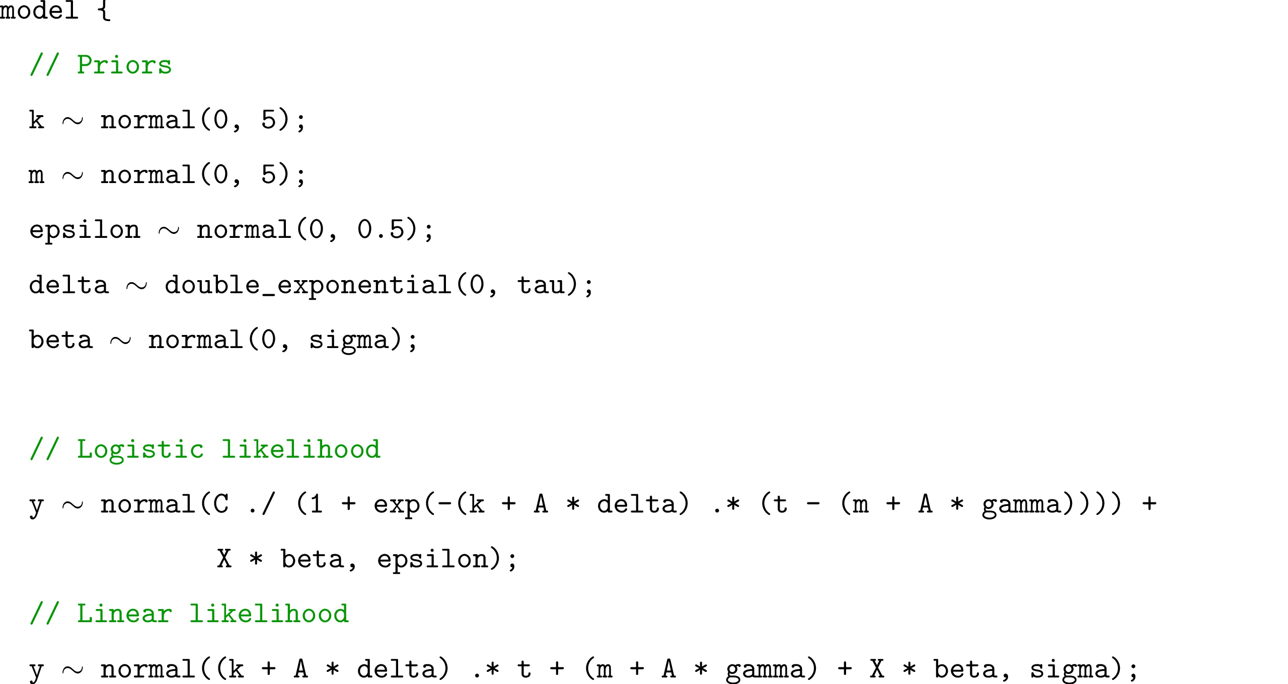
When the seasonality and holiday features for each observation are combined into a matrix X and the changepoint indicators a(t) in a matrix A, the entire model in (1) can be expressed in a few lines of Stan code (Carpenter et al. 2017), given in Listing 1. For model ﬁtting we use Stan’s L-BFGS to ﬁnd a maximum a posteriori estimate, but also can do

当每个观测的季节性和假日特征被组合成矩阵X和矩阵A中的变化点指标a（t）时，（1）中的整个模型可以用几行Stan代码表示（Carpenter等人。 2017），如清单1所示。对于模型配置，我们使用Stan的L-BFGS来确定最大后验估计，但也可以做

Listing 1: Example Stan code for our complete model.

清单1：完整模型的示例Stan代码。

}

full posterior inference to include model parameter uncertainty in the forecast uncertainty. Fig. 4 shows the Prophet model forecast to the Facebook events time series of Fig. 3. These forecasts were made on the same three dates as in Fig. 3, as before using only the data up to that date for the forecast. The Prophet forecast is able to predict both the weekly and yearly seasonalities, and unlike the baselines in Fig. 3, does not overreact to the holiday dip in the ﬁrst year. In the ﬁrst forecast, the Prophet model has slightly overﬁt the yearly seasonality given only one year of data. In the third forecast, the model has not yet learned that the trend has changed. Fig. 5 shows that a forecast incorporating the most recent three months of data exhibits the trend change (dashed line).

全后验推断包括模型参数不确定性在预测不确定性中的应用。图4显示了对图3的Facebook事件时间序列的Prophet模型预测。这些预测是在与图3相同的三个日期进行的，就像之前仅使用截至该日期的预测数据一样。先知预测能够预测每周和每年的季节性，与图3中的基线不同，它不会对第一年的假期下降做出过度反应。在第一次预测中，只有一年的数据，Prophet模型略微超过了年度季节性。在第三次预测中，该模型尚未了解趋势已发生变化。图5显示包含最近三个月数据的预测显示趋势变化（虚线）。

An important beneﬁt of the decomposable model is that it allows us to look at each component of the forecast separately. Fig. 6 shows the trend, weekly seasonality, and yearly seasonality components corresponding to the last forecast in Fig. 4. This provides a useful tool for analysts to gain insight into their forecasting problem, besides just producing a prediction.

可分解模型的一个重要好处是它允许我们分别查看预测的每个组成部分。图6示出了与图4中的最后预测相对应的趋势，每周季节性和年度季节性分量。除了产生预测外，这为分析师提供了一个有用的工具，可以深入了解他们的预测问题。

The parameters tau and sigma in Listing 1 are controls for the amount of regularization on the model changepoints and seasonality respectively. Regularization is important for both of these to avoid overﬁtting, however there likely is not enough historical data to select the best regularization parameters via cross-validation. We set default values that are appropriate for most forecasting problems, and when these parameters need to be optimized it happens with the analyst in the loop.

清单1中的参数tau和sigma分别是对模型变化点和季节性的正则化量的控制。正规化对于这两者都很重要，以避免过度拟合，但是可能没有足够的历史数据来通过交叉验证来选择最佳正则化参数。我们设置了适合大多数预测问题的默认值，当需要优化这些参数时，循环中的分析师就会发生这种情况。

Figure 4: Prophet forecasts corresponding to those of Fig. 3. As before, forecasts are grouped by day-of-week to visualize weekly seasonality.

图4：先知预测对应于图3的预测。和以前一样，预测按星期分组，以显示每周季节性。

Figure 5: Prophet forecast using all available data, including the interpolation of the historical data. Solid lines are in-sample ﬁt, dashed lines are out-of-sample forecast.

图5：先知预测使用所有可用数据，包括历史数据的插值。实线是样本内的虚线，虚线是样本外的预测。

Figure 6: Components of the Prophet forecast in Fig. 5.

图6：图5中先知预测的组成部分。

3.5 Analyst-in-the-Loop Modeling

3.5分析在环建模

Analysts making forecasts often have extensive domain knowledge about the quantity they are forecasting, but limited statistical knowledge. In the Prophet model speciﬁcation there are several places where analysts can alter the model to apply their expertise and external knowledge without requiring any understanding of the underlying statistics.

进行预测的分析师通常对他们预测的数量有广泛的领域知识，但统计知识有限。在先知模型规范中，分析师可以通过几个地方改变模型，以应用他们的专业知识和外部知识，而无需了解基础统计数据。

Capacities: Analysts may have external data for the total market size and can apply that knowledge directly by specifying capacities.

能力：分析师可能拥有总市场规模的外部数据，可以通过指定容量直接应用这些知识。

Changepoints: Known dates of changepoints, such as dates of product changes, can be directly speciﬁed.

变更点：可以直接指定变更点的已知日期，例如产品变更的日期。

Holidays and seasonality: Analysts that we work with have experience with which holidays impact growth in which regions, and they can directly input the relevant holiday dates and the applicable time scales of seasonality.

假期和季节性：我们合作的分析师有哪些假期影响哪些地区的增长，他们可以直接输入相关的假日日期和适用的季节性时间尺度。

With good visualization tools, analysts can use these parameters to improve the model ﬁt. When the model ﬁt is plotted over historical data, it is quickly apparent if there were changepoints that were missed by the automatic changepoint selection. The τ parameter is a single knob that can be turned to increase or decrease the trend ﬂexibility, and σ is a knob to increase or decrease the strength of the seasonality component. Visualization provides many other opportunities for fruitful human intervention: linear trend or logistic growth, identifying time scales of seasonality, and identifying outlying time periods that should be removed from ﬁtting are a few. All of these interventions can be made without statistical expertise, and are important ways for analysts to apply their insights or domain knowledge.

通过良好的可视化工具，分析人员可以使用这些参数来改进模型。当在历史数据上绘制模型时，很快就会发现自动变换点选择是否遗漏了变化点。τ参数是单个旋钮，可以转动以增加或减少趋势灵活性，σ是增加或减少季节性成分强度的旋钮。可视化为富有成效的人为干预提供了许多其他机会：线性趋势或后勤增长，确定季节性的时间尺度，以及识别应该从设置中删除的外围时间段等。所有这些干预都可以在没有统计专业知识的情况下进行，并且是分析师应用他们的见解或领域知识的重要途径。

The forecasting literature often makes the distinction between statistical forecasts, which are based on models ﬁt to historical data, and judgmental forecasts (also called managerial forecasts), which human experts produce using whatever process they have learned tends to work well for a speciﬁc time series. Each of these approaches has their advantages. Statistical forecasts require less domain knowledge and eﬀort from human forecasters, and they can scale to many forecasts very easily. Judgmental forecasts can include more information and be more responsive to changing conditions, but can require intensive work by analysts (Sanders 2005).

预测文献通常将基于模型与历史数据相关的统计预测与判断性预测（也称为管理预测）区分开来，人类专家使用他们学到的任何过程生成的预测往往适用于特定的时间序列。。这些方法中的每一种都有其优点。统计预测需要较少的领域知识和来自人类预报员的效果，并且它们可以非常容易地扩展到许多预测。判断预测可以包括更多信息，并且对变化的条件更敏感，但可能需要分析师的密集工作（Sanders，2005）。

Our analyst-in-the-loop modeling approach is an alternative approach that attempts to blend the advantages of statistical and judgmental forecasts by focusing analyst eﬀort on improving the model when necessary rather that directly producing forecasts through some unstated procedure. We ﬁnd that our approach closely resembles the “transform-visualizemodel” loop proposed by Wickham & Grolemund (2016), where the human domain knowledge is codiﬁed in an improved model after some iteration.

我们的分析员在环建模方法是一种替代方法，试图通过将分析师的工作重点放在必要时改进模型而不是通过一些未说明的程序直接产生预测来融合统计和判断预测的优势。我们发现我们的方法非常类似于Wickham＆Grolemund（2016）提出的“transform-visualizemodel”循环，其中人类领域知识在经过一些迭代后在改进的模型中进行了修改。

Typical scaling of forecasting would rely on fully automated procedures, but judgmental forecasts have been shown to be highly accurate in many applications (Lawrence et al. 2006). Our proposed approach lets analysts apply judgment to forecasts through a small set of intuitive model parameters and options, while retaining the ability to fall back on fully automated statistical forecasting when necessary. As of this writing we have only anecdotal empirical evidence for possible improvements to accuracy, but we look forward to future research which can evaluate the improvements analysts can have in a modelassisted setting.

预测的典型扩展将依赖于完全自动化的程序，但是在许多应用中已经证明判断性预测是高度准确的（Lawrence等人，2006）。我们提出的方法可以让分析师通过一小组直观的模型参数和选项对预测进行判断，同时保留在必要时依靠全自动统计预测的能力。在撰写本文时，我们只有可能提高准确性的经验证据，但我们期待未来的研究可以评估分析师在模式分类环境中可以获得的改进。

The ability to have an analyst-in-the-loop at scale relies critically on automatic evaluation of forecast quality and good visualization tools. We now describe how forecast evaluation can be automated to identify the most relevant forecasts for analyst input.

大规模分析在环中的能力主要依赖于预测质量的自动评估和良好的可视化工具。我们现在描述如何自动预测评估，以确定分析师输入的最相关预测。

4 Automating Evaluation of Forecasts

4自动评估预测

In this section we outline a procedure for automating forecast performance evaluation, by comparing various methods and identifying forecasts where manual intervention may be warranted. This section is agnostic to the forecasting method used and contains some bestpractices we have settled on while shipping production business forecasts across a variety of applications.

在本节中，我们概述了自动化预测绩效评估的程序，通过比较各种方法和确定可能需要人工干预的预测。本部分与所使用的预测方法无关，并包含我们在各种应用程序中生成生产业务预测时已确定的一些最佳实践。

4.1 Use of Baseline Forecasts

4.1基线预测的使用

When evaluating any forecasting procedure it is important to compare to a set of baseline methods. We prefer using simplistic forecasts that make strong assumptions about the underlying process but that can produce a reasonable forecast in practice. We have found it useful to compare simplistic models (last value and sample mean) as well as the automated forecasting procedures described in Section 2.

在评估任何预测过程时，与一组基线方法进行比较非常重要。我们更倾向于使用简单的预测，对基础流程做出强有力的假设，但这可以在实践中产生合理的预测。我们发现比较简单模型（最后值和样本均值）以及第2节中描述的自动预测程序很有用。

4.2 Modeling Forecast Accuracy

4.2建模预测准确性

Forecasts are made over a certain horizon, which we denote H. The horizon is the number of days in the future we care about forecasting – this is typically 30, 90, 180, or 365 days in our applications. Thus for any forecast with daily observations, we produce up to H estimates of future states that will each be associated with some error. We need to declare a forecasting objective to compare methods and track performance. Additionally, understanding how error-prone our forecasting procedure is can allow consumers of the forecasts in a business setting to determine whether to trust it at all.

预测是在某个范围内进行的，我们将其表示为H.地平线是我们关注预测的未来天数 - 在我们的应用程序中通常为30天，90天，180天或365天。因此，对于每日观测的任何预测，我们产生对未来状态的H估计，每个状态将与一些误差相关联。我们需要声明一个预测目标来比较方法和跟踪性能。此外，了解我们的预测程序如何容易出错，可以让业务环境中的预测消费者确定是否完全信任它。

Let ˆy( ) represent a forecast for time t made with historical information up to time T and d( ) be a distance metric such as mean absolute error, d( ) = . Choice of a distance function should be problem-speciﬁc. De Gooijer & Hyndman (2006) review several such error metrics – in practice we prefer mean absolute percentage error (MAPE) for its interpretability. We deﬁne the empirical accuracy of a forecast of (0 ] periods ahead of time T as:

令y（）表示对历史信息进行的时间t的预测直到时间T并且d（）是距离度量，例如平均绝对误差，d（）= 。距离函数的选择应该是问题特定的。De Gooijer＆Hyndman（2006）回顾了几个这样的误差指标 - 实际上我们更倾向于使用平均绝对百分误差（MAPE）来解释它。我们将提前预测（0 ）期间的经验准确性定义为：

In order to form an estimate of this accuracy and how it varies with h, it is common to specify a parametric model for the error term and to estimate its parameters from data. For instance if we were using an AR(1) model, y(t) = α + ( 1) + ν(t), we would assume that ν(t) ∼ Normal(0 2ν) and focus on estimating the variance term σ2ν from the data. Then we could form expectations using any distance function through simulation or by using an analytic expression for the expectation of the sum of the errors. Unfortunately these approaches only give correct estimates of error conditional on having speciﬁed the correct model for the process – a condition that is unlikely to hold in practice.

为了形成对该精度的估计以及它如何随h变化，通常为误差项指定参数模型并从数据中估计其参数。例如，如果我们使用AR（1）模型，y（t）=α+ （ 1）+ν（t），我们假设ν（t）〜正常（0 ν）并专注于估计来自数据的方差项σ2ν。然后，我们可以通过模拟使用任何距离函数或通过使用分析表达式来预期误差总和。不幸的是，这些方法只能给出正确的误差估计条件，条件是指定了过程的正确模型 - 这种情况在实践中不太可能存在。

We prefer to take a non-parametric approach to estimating expected errors that is applicable across models. The approach is similar to applying cross-validation to estimate out-of-sample error for models making predictions on i.i.d. data. Given a set of historical forecasts, we ﬁt a model of the expected error we would make at diﬀerent forecast horizons h:

我们倾向于采用非参数方法来估计适用于模型的预期误差。该方法类似于应用交叉验证来估计在i.i.d上进行预测的模型的样本外误差。数据。给定一组历史预测，我们得到一个模型，我们将在不同的预测视野中做出预期误差h：

This model should be ﬂexible but can impose some simple assumptions. First, the function should be locally smooth in h because we expect any mistakes we make on consecutive days to be relatively similar. Second, we may impose the assumption that the function should be weakly increasing in h, although this need not be the case for all forecast models. In practice, we use a local regression (Cleveland & Devlin 1988) or isotonic regression (Dykstra 1981) as ﬂexible non-parametric models of error curves.

这个模型应该是灵活的，但可以强加一些简单的假设。首先，函数在h中应该是局部平滑的，因为我们预计连续几天我们所犯的任何错误都会相对相似。其次，我们可以假设函数应该在h中微弱地增加，尽管并非所有预测模型都是如此。在实践中，我们使用局部回归（Cleveland＆Devlin 1988）或等渗回归（Dykstra 1981）作为灵敏的非参数误差曲线模型。

In order to generate historical forecast errors to ﬁt this model, we use a procedure we call simulated historical forecasts.

为了生成历史预测误差以使用该模型，我们使用称为模拟历史预测的过程。

4.3 Simulated Historical Forecasts

4.3模拟的历史预测

We would like to ﬁt the expected error model in (8) to perform model selection and evaluation. Unfortunately it is diﬃcult to use a method like cross validation because the observations are not exchangeable – we cannot simply randomly partition the data.

我们希望在（8）中找到预期的误差模型来执行模型选择和评估。不幸的是，使用像交叉验证这样的方法是很困难的，因为观察结果是不可交换的 - 我们不能简单地随机分割数据。

We use simulated historical forecasts (SHFs) by producing K forecasts at various cutoﬀ points in the history, chosen such that the horizons lie within the history and the total error can be evaluated. This procedure is based on classical “rolling origin” forecast evaluation procedures (Tashman 2000), but uses only a small sequence of cutoﬀ dates rather than making one forecast per historical date. The main advantage of using fewer simulated dates (rolling origin evaluation produces one forecast per date) is that it economizes on computation while providing less correlated accuracy measurements.

我们使用模拟历史预测（SHF），通过在历史中的各种cuto ff点产生K预测，选择使得视野位于历史中并且可以评估总误差。此程序基于经典的“滚动起源”预测评估程序（Tashman 2000），但仅使用一小部分cuto ff日期，而不是每个历史日期进行一次预测。使用较少模拟日期（滚动原点评估每个日期产生一个预测）的主要优点是它可以节省计算，同时提供较少相关的精度测量。

SHFs simulate the errors we would have made had we used this forecasting method at those points in the past. The forecasts in Figs. 3 and 4 are examples of SHFs. This method has the advantage of being simple, easy to explain to analysts and decision makers, and relatively uncontroversial for generating insight into forecast errors. There are two main issues to be aware of when using the SHF methodology to evaluate and compare forecasting approaches.

SHF模拟了我们在过去的那些点使用这种预测方法时可能会犯的错误。图中的预测。图3和4是SHF的示例。该方法具有简单，易于向分析人员和决策者解释的优点，并且对于生成对预测错误的洞察而言相对无可争议。使用SHF方法评估和比较预测方法时，需要注意两个主要问题。

First, the more simulated forecasts we make, the more correlated their estimates of error are. In the extreme case of a simulated forecast for each day in the history, the forecasts are unlikely to have changed much given an additional day of information and the errors from one day to the next would be nearly identical. On the other hand, if we make very few simulated forecasts then we have fewer observations of historical forecasting errors on which to base our model selection. As a heuristic, for a forecast horizon H, we generally make a simulated forecast every 2 periods. Although correlated estimates do not introduce bias into our estimation of model accuracy, they do produce less useful information and slow down forecast evaluation.

首先，我们制作的模拟预测越多，他们对误差的估计就越相关。在历史中每天的模拟预测的极端情况下，由于额外的一天信息，预测不太可能发生很大变化，并且从一天到下一天的误差几乎相同。另一方面，如果我们进行的模拟预测很少，那么我们对模型选择的历史预测误差的观察就会减少。作为启发式，对于预测范围H，我们通常在每个 2个时段进行模拟预测。虽然相关估计不会在我们对模型准确性的估计中引入偏差，但它们确实产生的信息较少，并且减缓了预测评估。

Second, forecasting methods can perform better or worse with more data. A longer history can lead to worse forecasts when the model is misspeciﬁed and we are overﬁtting the past, for example using the sample mean to forecast a time series with a trend.

其次，预测方法可以在更多数据的情况下表现更好或更差。较长的历史记录可能导致更糟糕的预测，当模型未指定并且我们过去时，例如使用样本均值来预测具有趋势的时间序列。

Fig. 7 shows our estimates of the function ξ(h), the expected mean absolute percentage error across the forecast period using LOESS, for the time series of Figs. 3 and 4. The estimate was made using nine simulated forecast dates, one per quarter beginning after the ﬁrst year. Prophet has lower prediction error across all forecast horizons. The Prophet forecasts were made with default settings, and tweaking the parameters could possibly further improve performance.

图7显示了我们对函数ξ（h）的估计，即使用LOESS的预测期间的预期平均绝对百分比误差，对于图7和图8的时间序列。 3和4。估算是使用九个模拟预测日期进行的，每个季度一个，从第一年开始。先知在所有预测视野中的预测误差较低。先知预测是使用默认设置进行的，调整参数可能会进一步提高性能。

When visualizing forecasts, we prefer to use points rather than lines to represent histor ical data, inasmuch as these represent precise measurements that are never interpolated. We then overlay lines with the forecasts. For SHFs, it is useful to visualize the errors the model has made at various horizons, both as a time series (as in Fig. 3) and aggregated over SHFs (as in Fig. 7).

在可视化预测时，我们更倾向于使用点而不是线来表示历史数据，因为这些数据代表了从未插值的精确测量。然后我们用预测覆盖线条。对于SHF，可视化模型在各种视野中所做的错误，既可以作为时间序列（如图3所示），也可以聚合在SHF上（如图7所示）。

Figure 7: Smoothed mean absolute percentage errors for the forecasting methods and time series of Figs. 3 and 4. Prophet forecasts had substantially lower prediction error than the other automated forecast methods.

图7：图1和图2的预测方法和时间序列的平滑平均绝对百分比误差。 3和4。先知预测的预测误差远低于其他自动预测方法。

Even for a single time series SHFs require many forecasts to be computed, and at scale we may want to forecast many diﬀerent metrics at many diﬀerent levels of aggregation. SHFs can be computed independently on separate machines as long as those machines can write to the same data store. We store our forecasts and associated errors in Hive or MySQL depending on their intended use.

即使对于单个时间序列，SHF也需要计算许多预测，并且在规模上我们可能希望在许多不同的聚合水平上预测许多不同的指标。只要这些机器可以写入同一个数据存储，SHF就可以在不同的机器上独立计算。我们根据预期用途将我们的预测和相关错误存储在Hive或MySQL中。

4.4 Identifying Large Forecast Errors

4.4识别大型预测错误

When there are too many forecasts for analysts to manually check each of them, it is important to be able to automatically identify forecasts that may be problematic. Automatically identifying bad forecasts allows analysts to use their limited time most eﬀectively, and to use their expertise to correct any issues. There are several ways that SHFs can be used to identify likely problems with the forecasts.

当分析师有太多预测手动检查每个预测时，能够自动识别可能存在问题的预测非常重要。自动识别不良预测允许分析师最有效地利用他们有限的时间，并使用他们的专业知识来纠正任何问题。有几种方法可以使用SHF来识别预测可能出现的问题。

- When the forecast has large errors relative to the baselines, the model may be mis

- 当预测相对于基线有较大误差时，模型可能是错误的

speciﬁed. Analysts can adjust the trend model or the seasonality, as needed.

SPECI网络版。分析师可根据需要调整趋势模型或季节性。

- Large errors for all methods on a particular date are suggestive of outliers. Analysts can identify outliers and remove them.

- 特定日期所有方法的大错误都暗示了异常值。分析师可以识别异常值并将其删除。

- When the SHF error for a method increases sharply from one cutoﬀ to the next, it could indicate that the data generating process has changed. Adding changepoints or modeling diﬀerent phases separately may address the issue.

- 当方法的SHF错误从一个cuto ff急剧增加到下一个cuto时，它可能表明数据生成过程已经改变。分别添加变更点或建模不同阶段可能会解决问题。

There are pathologies that cannot be easily corrected, but most of the issues that we have encountered can be corrected by specifying changepoints and removing outliers. These issues are easily identiﬁed and corrected once the forecast has been ﬂagged for review and visualized.

有些病症无法轻易纠正，但我们遇到的大多数问题都可以通过指定变更点和删除异常值来纠正。一旦预测被征集以供审查和可视化，这些问题很容易识别和纠正。

5 Conclusion

5结论

A major theme of forecasting at scale is that analysts with a variety of backgrounds must make more forecasts than they can do manually. The ﬁrst component of our forecasting system is the new model that we have developed over many iterations of forecasting a variety of data at Facebook. We use a simple, modular regression model that often works well with default parameters, and that allows analysts to select the components that are relevant to their forecasting problem and easily make adjustments as needed. The second component is a system for measuring and tracking forecast accuracy, and ﬂagging forecasts that should be checked manually to help analysts make incremental improvements. This is a critical component which allows analysts to identify when adjustments need to be made to the model or when an entirely diﬀerent model may be appropriate. Simple, adjustable models and scalable performance monitoring in combination allow a large number of analysts to forecast a large number and a variety of time series – what we consider forecasting at scale.

大规模预测的一个主要主题是具有不同背景的分析师必须做出比他们手动更多的预测。我们预测系统的第一个组成部分是我们在Facebook上预测各种数据的多次迭代中开发的新模型。我们使用简单的模块化回归模型，该模型通常可以很好地使用默认参数，并允许分析人员选择与其预测问题相关的组件，并根据需要轻松进行调整。第二个组件是用于测量和跟踪预测准确性的系统，以及应该手动检查以帮助分析师进行渐进式改进的预测。这是一个关键组件，它允许分析人员确定何时需要对模型进行调整，或者何时适合完全不同的模型。简单，可调整的模型和可扩展的性能监控相结合，允许大量分析师预测大量和各种时间序列 - 我们认为大规模预测。

6 Acknowledgements

6致谢

We thank Dan Merl for making the development of Prophet possible and for suggestions and insights throughout the development. We thank Dirk Eddelbuettel, Daniel Kaplan, Rob Hyndman, Alex Gilgur, and Lada Adamic for helpful reviews of this paper. We especially thank Rob Hyndman for insights connecting our work to judgemental forecasts.

我们感谢Dan Merl使Prophet的发展成为可能，并在整个开发过程中提出建议和见解。我们感谢Dirk Eddelbuettel，Daniel Kaplan，Rob Hyndman，Alex Gilgur和Lada Adamic对本文的有益评论。我们特别感谢Rob Hyndman将我们的工作与判断预测联系起来的见解。

FEATURED TAGS

FRIENDS